
LSTM Pytorch
Published:
![]()
Introduction to LSTM
In this notebook, I will build a character-level RNN/LSTM/GRU with PyTorch. The models will be able to generate new text based on the text from the book. The book called Grimms’ Fairy Tales by Jacob Grimm and Wilhelm Grimm. Datasets available at: https://www.kaggle.com/datasets/tschomacker/grimms-fairy-tales
Library
from collections import defaultdict
import copy
import random
import os
import shutil
from urllib.request import urlretrieve
import numpy as np
import matplotlib.pyplot as plt
from tqdm.notebook import tqdm
import torch
import torch.backends.cudnn as cudnn
import torch.nn as nn
import torch.nn.functional as F
import torch.optim
from torch.utils.data import Dataset, DataLoader
from tqdm import tqdm
from multiprocessing import Pool
cudnn.benchmark = True
from torchsummary import summary
import pickle
import pandas as pd
import time
import random
#fix seed for stable training
SEED = 42

random.seed(SEED)
np.random.seed(SEED)
torch.manual_seed(SEED)
torch.cuda.manual_seed(SEED)
torch.backends.cudnn.deterministic = True
Config
LEANRING_RATE = 0.001
#device
device = torch.device("cuda:0" if torch.cuda.is_available() else "cpu")
epochs = 30
Data Preporcessing
#read data
df_text = pd.read_csv("grimms_fairytales.csv")
list_all_text = []
for i in range(df_text.shape[0]):
  list_all_text.append(df_text['Text'][i])
#get all stories
text = " ".join(list_all_text)
#drop new line mask
text = text.replace("\n", "")
#int2char, which maps integers to characters ; char2int, which maps characters to unique integers
chars = tuple(set(text))
int2char = dict(enumerate(chars))
char2int = {ch: ii for ii, ch in int2char.items()}
#encode char to interge
encoded = np.array([char2int[ch] for ch in text])
# one-hot encoded for each character
def one_hot_encode(arr, n_labels):

    # Initialize the the encoded array
    one_hot = np.zeros((np.multiply(*arr.shape), n_labels), dtype=np.float32)

    # Fill the appropriate elements with ones
    one_hot[np.arange(one_hot.shape[0]), arr.flatten()] = 1.

    # Finally reshape it to get back to the original array
    one_hot = one_hot.reshape((*arr.shape, n_labels))

    return one_hot
# get data batch
def get_batches(arr, n_seqs, n_steps):
    '''Create a generator that returns batches of size
       n_seqs x n_steps from arr.

       Arguments
       ---------
       arr: Array you want to make batches from
       n_seqs: Batch size, the number of sequences per batch
       n_steps: Number of sequence steps per batch
    '''

    batch_size = n_seqs * n_steps
    n_batches = len(arr)//batch_size

    # Keep only enough characters to make full batches
    arr = arr[:n_batches * batch_size]
    # Reshape into n_seqs rows
    arr = arr.reshape((n_seqs, -1))

    for n in range(0, arr.shape[1], n_steps):
        # The features
        x = arr[:, n:n+n_steps]
        # The targets, shifted by one
        y = np.zeros_like(x)
        try:
            y[:, :-1], y[:, -1] = x[:, 1:], arr[:, n+n_steps]
        except IndexError:
            y[:, :-1], y[:, -1] = x[:, 1:], arr[:, 0]
        yield x, y
Build Model
class LSTM(nn.Module):

    def __init__(self, tokens, device, n_steps=100, n_hidden=256, n_layers=2, drop_prob=0.3):
        super().__init__()
        self.drop_prob = drop_prob
        self.n_layers = n_layers
        self.n_hidden = n_hidden
        self.device = device

        # creating character dictionaries
        self.chars = tokens
        self.int2char = dict(enumerate(self.chars))
        self.char2int = {ch: ii for ii, ch in self.int2char.items()}

        ## the LSTM
        self.lstm = nn.LSTM(len(self.chars), n_hidden, n_layers,
                            dropout=drop_prob, batch_first=True)

        ##  dropout layer
        self.dropout = nn.Dropout(drop_prob)

        ## fully-connected output layer
        self.fc = nn.Linear(n_hidden, len(self.chars))

        # initialize the weights
        self.init_weights()


    def forward(self, x, hc):
        ''' Forward pass through the network.
            These inputs are x, and the hidden/cell state `hc`. '''

        ## Get x, and the new hidden state (h, c) from the lstm
        x, (h, c) = self.lstm(x, hc)

        ## pass x through a droupout layer
        x = self.dropout(x)

        # Stack up LSTM outputs using view
        x = x.reshape(x.size()[0]*x.size()[1], self.n_hidden)

        ## put x through the fully-connected layer
        x = self.fc(x)

        # return x and the hidden state (h, c)
        return x, (h, c)

    def predict(self, char, h=None, device=device, top_k=5):
      ''' Given a character, predict the next character.

          Returns the predicted character and the hidden state.
      '''


      if h is None:
          h = self.init_hidden(1)

      x = np.array([[self.char2int[char]]])
      x = one_hot_encode(x, len(self.chars))
      inputs = torch.from_numpy(x)
      inputs = inputs.to(device)

      h = tuple([each.data for each in h])
      out, h = self.forward(inputs, h)

      p = F.softmax(out, dim=1).data
      p = p.to(device)

      if top_k is None:
          top_ch = np.arange(len(self.chars))
      else:
          p, top_ch = p.topk(top_k)
          top_ch = top_ch.cpu().numpy().squeeze()

      p = p.cpu().numpy().squeeze()
      char = np.random.choice(top_ch, p=p/p.sum())

      return self.int2char[char], h

    def init_weights(self):
        ''' Initialize weights for fully connected layer '''
        initrange = 0.1

        # Set bias tensor to all zeros
        self.fc.bias.data.fill_(0)
        # FC weights as random uniform
        self.fc.weight.data.uniform_(-1, 1)

    def init_hidden(self, n_seqs):
        ''' Initializes hidden state '''
        # Create two new tensors with sizes n_layers x n_seqs x n_hidden,
        # initialized to zero, for hidden state and cell state of LSTM
        weight = next(self.parameters()).data
        return (weight.new(self.n_layers, n_seqs, self.n_hidden).zero_(),
                weight.new(self.n_layers, n_seqs, self.n_hidden).zero_())
# define and print the model
model = LSTM(chars, device, n_hidden=512, n_layers=2)
print(model)
LSTM(
  (lstm): LSTM(77, 512, num_layers=2, batch_first=True, dropout=0.3)
  (dropout): Dropout(p=0.3, inplace=False)
  (fc): Linear(in_features=512, out_features=77, bias=True)
)
#optimizer
optimizer = torch.optim.Adam(model.parameters(), lr=LEANRING_RATE)
#loss function
criterion = nn.CrossEntropyLoss()
Training function
def epoch_time(start_time, end_time):
    elapsed_time = end_time - start_time
    elapsed_mins = int(elapsed_time / 60)
    elapsed_secs = int(elapsed_time - (elapsed_mins * 60))
    return elapsed_mins, elapsed_secs
def train(model, data, epochs=epochs, n_seqs=10, n_steps=50, opt=optimizer, criterion=criterion, device=device):
    '''
    Training a text generation network
    '''
    list_train_loss = []
    list_val_loss = []
    model.train()

    # create training and validation data
    val_frac = 0.1 # ratio train/val
    print_every = 50 #logging each n steps
    clip = 5 # gradient clipping
    best_valid_loss = float('inf') # best valid loss
    val_idx = int(len(data)*(1-val_frac))
    data, val_data = data[:val_idx], data[val_idx:]

    model.to(device)

    n_chars = len(model.chars)
    for e in tqdm(range(epochs)):
        start_time = time.monotonic()
        h = model.init_hidden(n_seqs)
        for x, y in get_batches(data, n_seqs, n_steps):

            # One-hot encode our data and make them Torch tensors
            x = one_hot_encode(x, n_chars)
            inputs, targets = torch.from_numpy(x), torch.from_numpy(y)

            inputs, targets = inputs.to(device), targets.to(device)

            # Creating new variables for the hidden state, otherwise
            # we'd backprop through the entire training history

            h = tuple([each.data for each in h])

            model.zero_grad()

            output, h = model.forward(inputs, h)
            loss = criterion(output, targets.view(n_seqs*n_steps))

            loss.backward()

            # `clip_grad_norm` helps prevent the exploding gradient problem in RNNs / LSTMs.
            nn.utils.clip_grad_norm_(model.parameters(), clip)

            opt.step()

        # validation
        val_h = model.init_hidden(n_seqs)
        val_losses = []
        for x, y in get_batches(val_data, n_seqs, n_steps):
            # One-hot encode our data and make them Torch tensors
            x = one_hot_encode(x, n_chars)
            x, y = torch.from_numpy(x), torch.from_numpy(y)

            # Creating new variables for the hidden state, otherwise
            # we'd backprop through the entire training history
            val_h = tuple([each.data for each in val_h])

            inputs, targets = x, y
            inputs, targets = inputs.to(device), targets.to(device)

            output, val_h = model.forward(inputs, val_h)
            val_loss = criterion(output, targets.view(n_seqs*n_steps))
        # save training and validation loss
        val_losses.append(val_loss.item())
        list_train_loss.append(loss.item())
        list_val_loss.append(np.mean(val_losses))
        #save best model
        if np.mean(val_losses) < best_valid_loss:
            best_valid_loss = np.mean(val_losses)
            torch.save(model.state_dict(), 'best-LSTM-model.pt')
        end_time = time.monotonic()

        epoch_mins, epoch_secs = epoch_time(start_time, end_time)

        print(f'\n Epoch: {e+1:02} | Epoch Time: {epoch_mins}m {epoch_secs}s')
        print(f'\tTrain Loss: {loss.item():.3f} ')
        print(f'\t Val. Loss: {np.mean(val_losses):.3f} ')
    return list_train_loss, list_val_loss
Start Training
#training model
n_seqs, n_steps = 128, 100
list_train_loss, list_val_loss = train(model, encoded,  n_seqs=n_seqs, n_steps=n_steps)
  3%|▎         | 1/30 [00:03<01:49,  3.77s/it]


 Epoch: 01 | Epoch Time: 0m 3s
	Train Loss: 2.825
	 Val. Loss: 2.798


  7%|▋         | 2/30 [00:06<01:35,  3.42s/it]


 Epoch: 02 | Epoch Time: 0m 3s
	Train Loss: 2.366
	 Val. Loss: 2.319


 10%|█         | 3/30 [00:10<01:30,  3.37s/it]


 Epoch: 03 | Epoch Time: 0m 3s
	Train Loss: 2.208
	 Val. Loss: 2.163


 13%|█▎        | 4/30 [00:13<01:24,  3.25s/it]


 Epoch: 04 | Epoch Time: 0m 3s
	Train Loss: 2.111
	 Val. Loss: 2.060


 17%|█▋        | 5/30 [00:16<01:19,  3.19s/it]


 Epoch: 05 | Epoch Time: 0m 3s
	Train Loss: 2.024
	 Val. Loss: 1.989


 20%|██        | 6/30 [00:19<01:15,  3.15s/it]


 Epoch: 06 | Epoch Time: 0m 3s
	Train Loss: 1.953
	 Val. Loss: 1.918


 23%|██▎       | 7/30 [00:22<01:12,  3.14s/it]


 Epoch: 07 | Epoch Time: 0m 3s
	Train Loss: 1.900
	 Val. Loss: 1.881


 27%|██▋       | 8/30 [00:25<01:08,  3.13s/it]


 Epoch: 08 | Epoch Time: 0m 3s
	Train Loss: 1.829
	 Val. Loss: 1.818


 30%|███       | 9/30 [00:28<01:05,  3.12s/it]


 Epoch: 09 | Epoch Time: 0m 3s
	Train Loss: 1.789
	 Val. Loss: 1.780


 33%|███▎      | 10/30 [00:31<01:02,  3.12s/it]


 Epoch: 10 | Epoch Time: 0m 3s
	Train Loss: 1.736
	 Val. Loss: 1.732


 37%|███▋      | 11/30 [00:35<00:59,  3.13s/it]


 Epoch: 11 | Epoch Time: 0m 3s
	Train Loss: 1.701
	 Val. Loss: 1.709


 40%|████      | 12/30 [00:38<00:56,  3.13s/it]


 Epoch: 12 | Epoch Time: 0m 3s
	Train Loss: 1.657
	 Val. Loss: 1.676


 43%|████▎     | 13/30 [00:41<00:53,  3.14s/it]


 Epoch: 13 | Epoch Time: 0m 3s
	Train Loss: 1.622
	 Val. Loss: 1.643


 47%|████▋     | 14/30 [00:44<00:50,  3.14s/it]


 Epoch: 14 | Epoch Time: 0m 3s
	Train Loss: 1.593
	 Val. Loss: 1.620


 50%|█████     | 15/30 [00:47<00:47,  3.14s/it]


 Epoch: 15 | Epoch Time: 0m 3s
	Train Loss: 1.557
	 Val. Loss: 1.606


 53%|█████▎    | 16/30 [00:50<00:44,  3.15s/it]


 Epoch: 16 | Epoch Time: 0m 3s
	Train Loss: 1.529
	 Val. Loss: 1.581


 57%|█████▋    | 17/30 [00:54<00:41,  3.16s/it]


 Epoch: 17 | Epoch Time: 0m 3s
	Train Loss: 1.498
	 Val. Loss: 1.559


 60%|██████    | 18/30 [00:57<00:37,  3.17s/it]


 Epoch: 18 | Epoch Time: 0m 3s
	Train Loss: 1.478
	 Val. Loss: 1.544


 63%|██████▎   | 19/30 [01:00<00:34,  3.15s/it]


 Epoch: 19 | Epoch Time: 0m 3s
	Train Loss: 1.450
	 Val. Loss: 1.544


 67%|██████▋   | 20/30 [01:03<00:31,  3.17s/it]


 Epoch: 20 | Epoch Time: 0m 3s
	Train Loss: 1.428
	 Val. Loss: 1.527


 70%|███████   | 21/30 [01:06<00:28,  3.16s/it]


 Epoch: 21 | Epoch Time: 0m 3s
	Train Loss: 1.406
	 Val. Loss: 1.517


 73%|███████▎  | 22/30 [01:09<00:25,  3.16s/it]


 Epoch: 22 | Epoch Time: 0m 3s
	Train Loss: 1.387
	 Val. Loss: 1.503


 77%|███████▋  | 23/30 [01:12<00:22,  3.15s/it]


 Epoch: 23 | Epoch Time: 0m 3s
	Train Loss: 1.373
	 Val. Loss: 1.501


 80%|████████  | 24/30 [01:16<00:18,  3.16s/it]


 Epoch: 24 | Epoch Time: 0m 3s
	Train Loss: 1.345
	 Val. Loss: 1.495


 83%|████████▎ | 25/30 [01:19<00:15,  3.17s/it]


 Epoch: 25 | Epoch Time: 0m 3s
	Train Loss: 1.330
	 Val. Loss: 1.488


 87%|████████▋ | 26/30 [01:22<00:12,  3.16s/it]


 Epoch: 26 | Epoch Time: 0m 3s
	Train Loss: 1.305
	 Val. Loss: 1.502


 90%|█████████ | 27/30 [01:25<00:09,  3.15s/it]


 Epoch: 27 | Epoch Time: 0m 3s
	Train Loss: 1.290
	 Val. Loss: 1.489


 93%|█████████▎| 28/30 [01:28<00:06,  3.14s/it]


 Epoch: 28 | Epoch Time: 0m 3s
	Train Loss: 1.273
	 Val. Loss: 1.491


 97%|█████████▋| 29/30 [01:32<00:03,  3.21s/it]


 Epoch: 29 | Epoch Time: 0m 3s
	Train Loss: 1.261
	 Val. Loss: 1.485


100%|██████████| 30/30 [01:35<00:00,  3.18s/it]


 Epoch: 30 | Epoch Time: 0m 3s
	Train Loss: 1.239
	 Val. Loss: 1.479
# plot training & validation loss
n_epochs = range(1, epochs+1)

# Plot and label the training and validation loss values
# Use our custom style
plt.style.use('ggplot')
plt.plot(n_epochs, list_train_loss, 'g', label='Training Loss')
plt.plot(n_epochs, list_val_loss,  'b', label='Validation Loss')

# Add in a title and axes labels
plt.title('Training and Validation Loss')
plt.xlabel('Epochs')
plt.ylabel('Loss')

# Set the tick locations
plt.xticks(range(1, epochs+1, 3))

# Display the plot
plt.legend(loc='best')
plt.show()
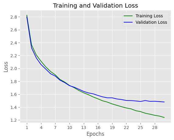
Both Training loss and validation loss gradually descrease, it shows that model learning process is effective.
Text Generation
# load the best checkpoint
model.load_state_dict(torch.load('best-LSTM-model.pt'))
<All keys matched successfully>
def text_generation(model, seq_length, input_text='a'):
    """
    Funcion to generate new character using trained deep model
    """
    model.eval()

    # First off, run through the prime characters
    chars = [ch for ch in input_text]
    h = model.init_hidden(1)
    for ch in input_text:
        char, h = model.predict(ch, h)

    chars.append(char)

    # Now pass in the previous character and get a new one
    for ii in range(seq_length):
        char, h = model.predict(chars[-1], h)
        chars.append(char)

    return ''.join(chars)
generate_text = text_generation(model, seq_length=500, input_text='story')
generate_text
'story winders; and as they were all sones towards to get out together for a bird singing, and was so to she had as tookingdown his wife; andhas she said tohimself, ‘If I can that was back to mark as have to stands.’ Then he went and looked another husband, but had brought in the child of the bride and croess. They said the peasants were all that he wished how it aspones that they could so, then he will go hometo her wood. Then the father had sicked a little sprong, help takeread any still the were to '
Generating text results are quite good since the results are very closed with true store. It proves that LSTM model is very good for sequene data.
GRU Model
class GRU(nn.Module):

    def __init__(self, tokens, device, n_steps=100, n_hidden=256, n_layers=2, drop_prob=0.3):
        super().__init__()
        self.drop_prob = drop_prob
        self.n_layers = n_layers
        self.n_hidden = n_hidden
        self.device = device

        # creating character dictionaries
        self.chars = tokens
        self.int2char = dict(enumerate(self.chars))
        self.char2int = {ch: ii for ii, ch in self.int2char.items()}

        ## the GRU
        self.gru = nn.GRU(len(self.chars), n_hidden, n_layers,
                            dropout=drop_prob, batch_first=True)

        ##  dropout layer
        self.dropout = nn.Dropout(drop_prob)

        ## fully-connected output layer
        self.fc = nn.Linear(n_hidden, len(self.chars))

        # initialize the weights
        self.init_weights()


    def forward(self, x, hc):
        ''' Forward pass through the network.
            These inputs are x, and the hidden/cell state `hc`. '''

        ## Get x, and the new hidden state (h, c) from the lstm
        x, h = self.gru(x, hc)

        ## pass x through a droupout layer
        x = self.dropout(x)

        # Stack up GRU outputs using view
        x = x.reshape(x.size()[0]*x.size()[1], self.n_hidden)

        ## put x through the fully-connected layer
        x = self.fc(x)

        # return x and the hidden state h
        return x, h

    def predict(self, char, h=None, device=device, top_k=5):
      ''' Given a character, predict the next character.

          Returns the predicted character and the hidden state.
      '''


      if h is None:
          h = self.init_hidden(1)

      x = np.array([[self.char2int[char]]])
      x = one_hot_encode(x, len(self.chars))
      inputs = torch.from_numpy(x)
      inputs = inputs.to(device)

      h = h.data
      h = h.to(device)

      out, h = self.forward(inputs, h)

      p = F.softmax(out, dim=1).data
      p = p.to(device)

      if top_k is None:
          top_ch = np.arange(len(self.chars))
      else:
          p, top_ch = p.topk(top_k)
          top_ch = top_ch.cpu().numpy().squeeze()

      p = p.cpu().numpy().squeeze()
      char = np.random.choice(top_ch, p=p/p.sum())

      return self.int2char[char], h

    def init_weights(self):
        ''' Initialize weights for fully connected layer '''
        initrange = 0.1

        # Set bias tensor to all zeros
        self.fc.bias.data.fill_(0)
        # FC weights as random uniform
        self.fc.weight.data.uniform_(-1, 1)

    def init_hidden(self, n_seqs):
        ''' Initializes hidden state '''
        # Create two new tensors with sizes n_layers x n_seqs x n_hidden,
        # initialized to zero, for hidden state and cell state of LSTM
        weight = next(self.parameters()).data
        return weight.new(self.n_layers, n_seqs, self.n_hidden).zero_()#, #weight.new(self.n_layers, n_seqs, self.n_hidden).zero_())
# define and print the model
model = GRU(chars, device, n_hidden=512, n_layers=2)
model = model.to(device)
print(model)
GRU(
  (gru): GRU(77, 512, num_layers=2, batch_first=True, dropout=0.3)
  (dropout): Dropout(p=0.3, inplace=False)
  (fc): Linear(in_features=512, out_features=77, bias=True)
)
#optimizer
optimizer = torch.optim.Adam(model.parameters(), lr=LEANRING_RATE)
#loss function
criterion = nn.CrossEntropyLoss()
def train_gru(model, data, epochs=epochs, n_seqs=10, n_steps=50, opt=optimizer, criterion=criterion, device=device):
    '''
    Training a text generation network
    '''
    list_train_loss = []
    list_val_loss = []
    model.train()

    # create training and validation data
    val_frac = 0.1 # ratio train/val
    print_every = 50 #logging each n steps
    clip = 5 # gradient clipping
    best_valid_loss = float('inf') # best valid loss
    val_idx = int(len(data)*(1-val_frac))
    data, val_data = data[:val_idx], data[val_idx:]

    model.to(device)

    n_chars = len(model.chars)
    for e in tqdm(range(epochs)):
        start_time = time.monotonic()
        h = model.init_hidden(n_seqs)

        for x, y in get_batches(data, n_seqs, n_steps):

            # One-hot encode our data and make them Torch tensors
            x = one_hot_encode(x, n_chars)
            inputs, targets = torch.from_numpy(x), torch.from_numpy(y)

            inputs, targets = inputs.to(device), targets.to(device)

            # Creating new variables for the hidden state, otherwise
            # we'd backprop through the entire training history
            h = h.data

            model.zero_grad()

            output, h = model.forward(inputs, h)
            loss = criterion(output, targets.view(n_seqs*n_steps))

            loss.backward()

            # clip_grad_norm` helps prevent the exploding gradient problem in RNNs / LSTMs.
            nn.utils.clip_grad_norm_(model.parameters(), clip)

            opt.step()

        # validation
        val_h = model.init_hidden(n_seqs)
        val_losses = []
        for x, y in get_batches(val_data, n_seqs, n_steps):
            # One-hot encode our data and make them Torch tensors
            x = one_hot_encode(x, n_chars)
            x, y = torch.from_numpy(x), torch.from_numpy(y)

            # Creating new variables for the hidden state, otherwise
            # we'd backprop through the entire training history
            # val_h = tuple([each.data for each in val_h])
            val_h = val_h.data

            inputs, targets = x, y
            inputs, targets = inputs.to(device), targets.to(device)

            output, val_h = model.forward(inputs, val_h)
            val_loss = criterion(output, targets.view(n_seqs*n_steps))
        # save training and validation loss
        val_losses.append(val_loss.item())
        list_train_loss.append(loss.item())
        list_val_loss.append(np.mean(val_losses))
        #save best model
        if np.mean(val_losses) < best_valid_loss:
            best_valid_loss = np.mean(val_losses)
            torch.save(model.state_dict(), 'best-GRU-model.pt')
        end_time = time.monotonic()

        epoch_mins, epoch_secs = epoch_time(start_time, end_time)

        print(f'\n Epoch: {e+1:02} | Epoch Time: {epoch_mins}m {epoch_secs}s')
        print(f'\tTrain Loss: {loss.item():.3f} ')
        print(f'\t Val. Loss: {np.mean(val_losses):.3f} ')
    return list_train_loss, list_val_loss
#training model
n_seqs, n_steps = 128, 100
list_train_loss, list_val_loss = train_gru(model, encoded, n_seqs=n_seqs, n_steps=n_steps)
  3%|▎         | 1/30 [00:02<01:16,  2.65s/it]


 Epoch: 01 | Epoch Time: 0m 2s
	Train Loss: 2.468
	 Val. Loss: 2.408


  7%|▋         | 2/30 [00:05<01:14,  2.65s/it]


 Epoch: 02 | Epoch Time: 0m 2s
	Train Loss: 2.230
	 Val. Loss: 2.176


 10%|█         | 3/30 [00:07<01:11,  2.66s/it]


 Epoch: 03 | Epoch Time: 0m 2s
	Train Loss: 2.131
	 Val. Loss: 2.082


 13%|█▎        | 4/30 [00:10<01:09,  2.66s/it]


 Epoch: 04 | Epoch Time: 0m 2s
	Train Loss: 2.059
	 Val. Loss: 2.011


 17%|█▋        | 5/30 [00:13<01:06,  2.67s/it]


 Epoch: 05 | Epoch Time: 0m 2s
	Train Loss: 1.988
	 Val. Loss: 1.945


 20%|██        | 6/30 [00:15<01:03,  2.67s/it]


 Epoch: 06 | Epoch Time: 0m 2s
	Train Loss: 1.926
	 Val. Loss: 1.894


 23%|██▎       | 7/30 [00:18<01:01,  2.67s/it]


 Epoch: 07 | Epoch Time: 0m 2s
	Train Loss: 1.859
	 Val. Loss: 1.846


 27%|██▋       | 8/30 [00:21<00:58,  2.68s/it]


 Epoch: 08 | Epoch Time: 0m 2s
	Train Loss: 1.812
	 Val. Loss: 1.805


 30%|███       | 9/30 [00:24<00:56,  2.68s/it]


 Epoch: 09 | Epoch Time: 0m 2s
	Train Loss: 1.765
	 Val. Loss: 1.768


 33%|███▎      | 10/30 [00:26<00:53,  2.69s/it]


 Epoch: 10 | Epoch Time: 0m 2s
	Train Loss: 1.728
	 Val. Loss: 1.734


 37%|███▋      | 11/30 [00:29<00:51,  2.69s/it]


 Epoch: 11 | Epoch Time: 0m 2s
	Train Loss: 1.686
	 Val. Loss: 1.713


 40%|████      | 12/30 [00:32<00:48,  2.69s/it]


 Epoch: 12 | Epoch Time: 0m 2s
	Train Loss: 1.663
	 Val. Loss: 1.677


 43%|████▎     | 13/30 [00:34<00:45,  2.69s/it]


 Epoch: 13 | Epoch Time: 0m 2s
	Train Loss: 1.624
	 Val. Loss: 1.657


 47%|████▋     | 14/30 [00:37<00:43,  2.70s/it]


 Epoch: 14 | Epoch Time: 0m 2s
	Train Loss: 1.596
	 Val. Loss: 1.640


 50%|█████     | 15/30 [00:40<00:40,  2.70s/it]


 Epoch: 15 | Epoch Time: 0m 2s
	Train Loss: 1.573
	 Val. Loss: 1.624


 53%|█████▎    | 16/30 [00:42<00:37,  2.70s/it]


 Epoch: 16 | Epoch Time: 0m 2s
	Train Loss: 1.550
	 Val. Loss: 1.605


 57%|█████▋    | 17/30 [00:45<00:35,  2.70s/it]


 Epoch: 17 | Epoch Time: 0m 2s
	Train Loss: 1.527
	 Val. Loss: 1.592


 60%|██████    | 18/30 [00:48<00:32,  2.71s/it]


 Epoch: 18 | Epoch Time: 0m 2s
	Train Loss: 1.517
	 Val. Loss: 1.571


 63%|██████▎   | 19/30 [00:51<00:29,  2.70s/it]


 Epoch: 19 | Epoch Time: 0m 2s
	Train Loss: 1.486
	 Val. Loss: 1.558


 67%|██████▋   | 20/30 [00:53<00:27,  2.71s/it]


 Epoch: 20 | Epoch Time: 0m 2s
	Train Loss: 1.468
	 Val. Loss: 1.552


 70%|███████   | 21/30 [00:56<00:24,  2.70s/it]


 Epoch: 21 | Epoch Time: 0m 2s
	Train Loss: 1.452
	 Val. Loss: 1.552


 73%|███████▎  | 22/30 [00:59<00:21,  2.71s/it]


 Epoch: 22 | Epoch Time: 0m 2s
	Train Loss: 1.436
	 Val. Loss: 1.533


 77%|███████▋  | 23/30 [01:01<00:19,  2.72s/it]


 Epoch: 23 | Epoch Time: 0m 2s
	Train Loss: 1.421
	 Val. Loss: 1.528


 80%|████████  | 24/30 [01:04<00:16,  2.72s/it]


 Epoch: 24 | Epoch Time: 0m 2s
	Train Loss: 1.400
	 Val. Loss: 1.519


 83%|████████▎ | 25/30 [01:07<00:13,  2.70s/it]


 Epoch: 25 | Epoch Time: 0m 2s
	Train Loss: 1.386
	 Val. Loss: 1.520


 87%|████████▋ | 26/30 [01:10<00:10,  2.71s/it]


 Epoch: 26 | Epoch Time: 0m 2s
	Train Loss: 1.365
	 Val. Loss: 1.510


 90%|█████████ | 27/30 [01:12<00:08,  2.71s/it]


 Epoch: 27 | Epoch Time: 0m 2s
	Train Loss: 1.358
	 Val. Loss: 1.508


 93%|█████████▎| 28/30 [01:15<00:05,  2.72s/it]


 Epoch: 28 | Epoch Time: 0m 2s
	Train Loss: 1.344
	 Val. Loss: 1.502


 97%|█████████▋| 29/30 [01:18<00:02,  2.73s/it]


 Epoch: 29 | Epoch Time: 0m 2s
	Train Loss: 1.330
	 Val. Loss: 1.501


100%|██████████| 30/30 [01:20<00:00,  2.70s/it]


 Epoch: 30 | Epoch Time: 0m 2s
	Train Loss: 1.319
	 Val. Loss: 1.513
# plot training & validation loss
n_epochs = range(1, epochs+1)

# Plot and label the training and validation loss values
# Use our custom style
plt.style.use('ggplot')
plt.plot(n_epochs, list_train_loss, 'g', label='Training Loss')
plt.plot(n_epochs, list_val_loss,  'b', label='Validation Loss')

# Add in a title and axes labels
plt.title('Training and Validation Loss for GRU model')
plt.xlabel('Epochs')
plt.ylabel('Loss')

# Set the tick locations
plt.xticks(range(1, epochs+1, 3))

# Display the plot
plt.legend(loc='best')
plt.show()
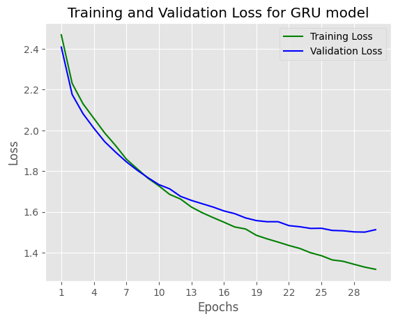
Comparing to LSTM model, GRU model loss slightly increases: from: 1.479 to 1.513
Text Generation using GRU
# load the best checkpoint
model.load_state_dict(torch.load('best-GRU-model.pt'))
<All keys matched successfully>
generate_text = text_generation(model, seq_length=500, input_text='story')
generate_text
'story we that all sister on,but he wished to hear and crossed his word four huntsman. ‘Ah! would be all were aring, and as he should be seen for the tailor. When the well plated that he was to see the boat, and happened, that the father went totheir first. ‘And you were something with me to heapt as have breen the forest the stood, and set over he was asked him word to say, and she were to live and was asked how it, and therower she had saded asked him what the feast asked him for a sold, which saw th'
Comparing with LSTM model, GRU model is less complexity but the text generating result is still quite good.
RNN Model
class RNN(nn.Module):

    def __init__(self, tokens, device, n_steps=100, n_hidden=256, n_layers=2, drop_prob=0.3):
        super().__init__()
        self.drop_prob = drop_prob
        self.n_layers = n_layers
        self.n_hidden = n_hidden
        self.device = device

        # creating character dictionaries
        self.chars = tokens
        self.int2char = dict(enumerate(self.chars))
        self.char2int = {ch: ii for ii, ch in self.int2char.items()}

        ## the RNN
        self.rnn = nn.RNN(len(self.chars), n_hidden, n_layers,
                            dropout=drop_prob, batch_first=True)

        ##  dropout layer
        self.dropout = nn.Dropout(drop_prob)

        ## fully-connected output layer
        self.fc = nn.Linear(n_hidden, len(self.chars))

        # initialize the weights
        self.init_weights()


    def forward(self, x, hc):
        ''' Forward pass through the network.
            These inputs are x, and the hidden/cell state `hc`. '''

        ## Get x, and the new hidden state (h, c) from the lstm
        x, h = self.rnn(x, hc)

        ## pass x through a droupout layer
        x = self.dropout(x)

        # Stack up GRU outputs using view
        x = x.reshape(x.size()[0]*x.size()[1], self.n_hidden)

        ## put x through the fully-connected layer
        x = self.fc(x)

        # return x and the hidden state h
        return x, h

    def predict(self, char, h=None, device=device, top_k=5):
      ''' Given a character, predict the next character.

          Returns the predicted character and the hidden state.
      '''


      if h is None:
          h = self.init_hidden(1)

      x = np.array([[self.char2int[char]]])
      x = one_hot_encode(x, len(self.chars))
      inputs = torch.from_numpy(x)
      inputs = inputs.to(device)

      h = h.data
      h = h.to(device)

      out, h = self.forward(inputs, h)

      p = F.softmax(out, dim=1).data
      p = p.to(device)

      if top_k is None:
          top_ch = np.arange(len(self.chars))
      else:
          p, top_ch = p.topk(top_k)
          top_ch = top_ch.cpu().numpy().squeeze()

      p = p.cpu().numpy().squeeze()
      char = np.random.choice(top_ch, p=p/p.sum())

      return self.int2char[char], h

    def init_weights(self):
        ''' Initialize weights for fully connected layer '''
        initrange = 0.1

        # Set bias tensor to all zeros
        self.fc.bias.data.fill_(0)
        # FC weights as random uniform
        self.fc.weight.data.uniform_(-1, 1)

    def init_hidden(self, n_seqs):
        ''' Initializes hidden state '''
        # Create two new tensors with sizes n_layers x n_seqs x n_hidden,
        # initialized to zero, for hidden state and cell state of LSTM
        weight = next(self.parameters()).data
        return weight.new(self.n_layers, n_seqs, self.n_hidden).zero_()#, #weight.new(self.n_layers, n_seqs, self.n_hidden).zero_())
# define and print the model
model = RNN(chars, device, n_hidden=512, n_layers=2)
model = model.to(device)
print(model)
RNN(
  (rnn): RNN(77, 512, num_layers=2, batch_first=True, dropout=0.3)
  (dropout): Dropout(p=0.3, inplace=False)
  (fc): Linear(in_features=512, out_features=77, bias=True)
)
def train_rnn(model, data, epochs=epochs, n_seqs=10, n_steps=50, opt=optimizer, criterion=criterion, device=device):
    '''
    Training a text generation network
    '''
    list_train_loss = []
    list_val_loss = []
    model.train()

    # create training and validation data
    val_frac = 0.1 # ratio train/val
    print_every = 50 #logging each n steps
    clip = 5 # gradient clipping
    best_valid_loss = float('inf') # best valid loss
    val_idx = int(len(data)*(1-val_frac))
    data, val_data = data[:val_idx], data[val_idx:]

    model.to(device)

    n_chars = len(model.chars)
    for e in tqdm(range(epochs)):
        start_time = time.monotonic()
        h = model.init_hidden(n_seqs)

        for x, y in get_batches(data, n_seqs, n_steps):

            # One-hot encode our data and make them Torch tensors
            x = one_hot_encode(x, n_chars)
            inputs, targets = torch.from_numpy(x), torch.from_numpy(y)

            inputs, targets = inputs.to(device), targets.to(device)

            # Creating new variables for the hidden state, otherwise
            # we'd backprop through the entire training history
            h = h.data

            model.zero_grad()

            output, h = model.forward(inputs, h)
            loss = criterion(output, targets.view(n_seqs*n_steps))

            loss.backward()

            # clip_grad_norm` helps prevent the exploding gradient problem in RNNs / LSTMs.
            nn.utils.clip_grad_norm_(model.parameters(), clip)

            opt.step()

        # validation
        val_h = model.init_hidden(n_seqs)
        val_losses = []
        for x, y in get_batches(val_data, n_seqs, n_steps):
            # One-hot encode our data and make them Torch tensors
            x = one_hot_encode(x, n_chars)
            x, y = torch.from_numpy(x), torch.from_numpy(y)

            # Creating new variables for the hidden state, otherwise
            # we'd backprop through the entire training history
            # val_h = tuple([each.data for each in val_h])
            val_h = val_h.data

            inputs, targets = x, y
            inputs, targets = inputs.to(device), targets.to(device)

            output, val_h = model.forward(inputs, val_h)
            val_loss = criterion(output, targets.view(n_seqs*n_steps))
        # save training and validation loss
        val_losses.append(val_loss.item())
        list_train_loss.append(loss.item())
        list_val_loss.append(np.mean(val_losses))
        #save best model
        if np.mean(val_losses) < best_valid_loss:
            best_valid_loss = np.mean(val_losses)
            torch.save(model.state_dict(), 'best-RNN-model.pt')
        end_time = time.monotonic()

        epoch_mins, epoch_secs = epoch_time(start_time, end_time)

        print(f'\n Epoch: {e+1:02} | Epoch Time: {epoch_mins}m {epoch_secs}s')
        print(f'\tTrain Loss: {loss.item():.3f} ')
        print(f'\t Val. Loss: {np.mean(val_losses):.3f} ')
    return list_train_loss, list_val_loss
#optimizer
optimizer = torch.optim.Adam(model.parameters(), lr=LEANRING_RATE)
#loss function
criterion = nn.CrossEntropyLoss()
#input and ouput RNN and GRU is same, so we can utilize training function from GRU
n_seqs, n_steps = 128, 100
list_train_loss, list_val_loss = train_rnn(model, encoded, opt=optimizer, criterion=criterion, n_seqs=n_seqs, n_steps=n_steps)
  3%|▎         | 1/30 [00:01<00:30,  1.07s/it]


 Epoch: 01 | Epoch Time: 0m 1s
	Train Loss: 2.233
	 Val. Loss: 2.188


  7%|▋         | 2/30 [00:02<00:29,  1.07s/it]


 Epoch: 02 | Epoch Time: 0m 1s
	Train Loss: 2.158
	 Val. Loss: 2.105


 10%|█         | 3/30 [00:03<00:28,  1.07s/it]


 Epoch: 03 | Epoch Time: 0m 1s
	Train Loss: 2.133
	 Val. Loss: 2.088


 13%|█▎        | 4/30 [00:04<00:27,  1.08s/it]


 Epoch: 04 | Epoch Time: 0m 1s
	Train Loss: 2.112
	 Val. Loss: 2.072


 17%|█▋        | 5/30 [00:05<00:27,  1.08s/it]


 Epoch: 05 | Epoch Time: 0m 1s
	Train Loss: 2.110
	 Val. Loss: 2.058


 20%|██        | 6/30 [00:06<00:25,  1.08s/it]


 Epoch: 06 | Epoch Time: 0m 1s
	Train Loss: 2.093
	 Val. Loss: 2.063


 23%|██▎       | 7/30 [00:07<00:24,  1.08s/it]


 Epoch: 07 | Epoch Time: 0m 1s
	Train Loss: 2.082
	 Val. Loss: 2.048


 27%|██▋       | 8/30 [00:08<00:23,  1.08s/it]


 Epoch: 08 | Epoch Time: 0m 1s
	Train Loss: 2.076
	 Val. Loss: 2.046


 30%|███       | 9/30 [00:09<00:22,  1.08s/it]


 Epoch: 09 | Epoch Time: 0m 1s
	Train Loss: 2.082
	 Val. Loss: 2.046


 33%|███▎      | 10/30 [00:10<00:21,  1.08s/it]


 Epoch: 10 | Epoch Time: 0m 1s
	Train Loss: 2.070
	 Val. Loss: 2.036


 37%|███▋      | 11/30 [00:11<00:20,  1.07s/it]


 Epoch: 11 | Epoch Time: 0m 1s
	Train Loss: 2.072
	 Val. Loss: 2.045


 40%|████      | 12/30 [00:12<00:19,  1.07s/it]


 Epoch: 12 | Epoch Time: 0m 1s
	Train Loss: 2.070
	 Val. Loss: 2.030


 43%|████▎     | 13/30 [00:13<00:18,  1.06s/it]


 Epoch: 13 | Epoch Time: 0m 1s
	Train Loss: 2.070
	 Val. Loss: 2.035


 47%|████▋     | 14/30 [00:15<00:16,  1.06s/it]


 Epoch: 14 | Epoch Time: 0m 1s
	Train Loss: 2.063
	 Val. Loss: 2.037


 50%|█████     | 15/30 [00:16<00:15,  1.06s/it]


 Epoch: 15 | Epoch Time: 0m 1s
	Train Loss: 2.066
	 Val. Loss: 2.032


 53%|█████▎    | 16/30 [00:17<00:14,  1.06s/it]


 Epoch: 16 | Epoch Time: 0m 1s
	Train Loss: 2.063
	 Val. Loss: 2.032


 57%|█████▋    | 17/30 [00:18<00:13,  1.07s/it]


 Epoch: 17 | Epoch Time: 0m 1s
	Train Loss: 2.062
	 Val. Loss: 2.025


 60%|██████    | 18/30 [00:19<00:12,  1.07s/it]


 Epoch: 18 | Epoch Time: 0m 1s
	Train Loss: 2.056
	 Val. Loss: 2.031


 63%|██████▎   | 19/30 [00:20<00:11,  1.07s/it]


 Epoch: 19 | Epoch Time: 0m 1s
	Train Loss: 2.056
	 Val. Loss: 2.030


 67%|██████▋   | 20/30 [00:21<00:10,  1.07s/it]


 Epoch: 20 | Epoch Time: 0m 1s
	Train Loss: 2.055
	 Val. Loss: 2.025


 70%|███████   | 21/30 [00:22<00:09,  1.07s/it]


 Epoch: 21 | Epoch Time: 0m 1s
	Train Loss: 2.049
	 Val. Loss: 2.020


 73%|███████▎  | 22/30 [00:23<00:08,  1.07s/it]


 Epoch: 22 | Epoch Time: 0m 1s
	Train Loss: 2.048
	 Val. Loss: 2.020


 77%|███████▋  | 23/30 [00:24<00:07,  1.07s/it]


 Epoch: 23 | Epoch Time: 0m 1s
	Train Loss: 2.046
	 Val. Loss: 2.032


 80%|████████  | 24/30 [00:25<00:06,  1.06s/it]


 Epoch: 24 | Epoch Time: 0m 1s
	Train Loss: 2.041
	 Val. Loss: 2.024


 83%|████████▎ | 25/30 [00:26<00:05,  1.06s/it]


 Epoch: 25 | Epoch Time: 0m 1s
	Train Loss: 2.049
	 Val. Loss: 2.026


 87%|████████▋ | 26/30 [00:27<00:04,  1.07s/it]


 Epoch: 26 | Epoch Time: 0m 1s
	Train Loss: 2.049
	 Val. Loss: 2.019


 90%|█████████ | 27/30 [00:28<00:03,  1.08s/it]


 Epoch: 27 | Epoch Time: 0m 1s
	Train Loss: 2.046
	 Val. Loss: 2.018


 93%|█████████▎| 28/30 [00:29<00:02,  1.07s/it]


 Epoch: 28 | Epoch Time: 0m 1s
	Train Loss: 2.044
	 Val. Loss: 2.023


 97%|█████████▋| 29/30 [00:31<00:01,  1.07s/it]


 Epoch: 29 | Epoch Time: 0m 1s
	Train Loss: 2.044
	 Val. Loss: 2.018


100%|██████████| 30/30 [00:32<00:00,  1.07s/it]


 Epoch: 30 | Epoch Time: 0m 1s
	Train Loss: 2.040
	 Val. Loss: 2.015
# plot training & validation loss
n_epochs = range(1, epochs+1)

# Plot and label the training and validation loss values
# Use our custom style
plt.style.use('ggplot')
plt.plot(n_epochs, list_train_loss, 'g', label='Training Loss')
plt.plot(n_epochs, list_val_loss,  'b', label='Validation Loss')

# Add in a title and axes labels
plt.title('Training and Validation Loss for RNN model')
plt.xlabel('Epochs')
plt.ylabel('Loss')

# Set the tick locations
plt.xticks(range(1, epochs+1, 3))

# Display the plot
plt.legend(loc='best')
plt.show()
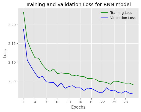
Comparing to LSTM model val loss (1.479) , GRU model val loss (1.513), RNN model val loss (2.015) is not good as 2 above models, it prove that RNN model is easy to be gradient vanishing.
Text Generation using RNN
# load the best checkpoint
model.load_state_dict(torch.load('best-RNN-model.pt'))
<All keys matched successfully>
generate_text = text_generation(model, seq_length=500, input_text='story')
generate_text
'story,’ se wal ane, what aid ther wof to maite and st one the washe tho gove mee shim, and tisht whathe toree tase, and at her hare, and harde hin timen to soo die, ‘Whar have aid one anoul to ther, ald tain so fors wis, he wile hares, and we tha gha butt he he are th there tore the bat hit watlit, hed her was se cound to kn the wirle th ter boo merang, an thous tere anding ono he anger, and harde the tall gat taind she said, ard wer welle, as wat then inther, and her the ser and har tore the so fan t'
###Conclusion
LSTM Text Generating results:
story winders; and as they were all sones towards to get out together for a bird singing, and was so to she had as tookingdown his wife; andhas she said tohimself, ‘If I can that was back to mark as have to stands.’ Then he went and looked another husband, but had brought in the child of the bride and croess. They said the peasants were all that he wished how it aspones that they could so, then he will go hometo her wood. Then the father had sicked a little sprong, help takeread any still the were to
GRU Text Generating results:
story we that all sister on,but he wished to hear and crossed his word four huntsman. ‘Ah! would be all were aring, and as he should be seen for the tailor. When the well plated that he was to see the boat, and happened, that the father went totheir first. ‘And you were something with me to heapt as have breen the forest the stood, and set over he was asked him word to say, and she were to live and was asked how it, and therower she had saded asked him what the feast asked him for a sold, which saw th
RNN Text Generating results:
story,’ se wal ane, what aid ther wof to maite and st one the washe tho gove mee shim, and tisht whathe toree tase, and at her hare, and harde hin timen to soo die, ‘Whar have aid one anoul to ther, ald tain so fors wis, he wile hares, and we tha gha butt he he are th there tore the bat hit watlit, hed her was se cound to kn the wirle th ter boo merang, an thous tere anding ono he anger, and harde the tall gat taind she said, ard wer welle, as wat then inther, and her the ser and har tore the so fan t
Conclusion:
- After training LSTM, GRU and RNN for task text generation: RNN model result is not good as LSTM or GRU since RNN model faces vanishing gradient.
- GRU & LSTM achieved good results both for validation loss and text generating result.
.
###Future Imporvement
- Text generation using Transfomer: a SOTA architecture for many domains such as NLP, Vision, Audio.
- Word-level approach
- Apply SOTA text generation pretrained model such as GPT-3.5 or BERT-family models